Subtitle: Building our rendering on solidly shaky grounds.
Physically-Based Rendering has won. There is no question about it, after an initial period of reluctance, even artists have been converted and I don't think you can find many rendering systems nowadays, either offline or real-time, that hasn't embraced PBR. And PBR proved itself to even be able to adapt to multiple art styles, outside strict adherence to photorealism.
But, really, how much physics is there in our PBR renderers? Let's have a look.
- Optics and Photometry.
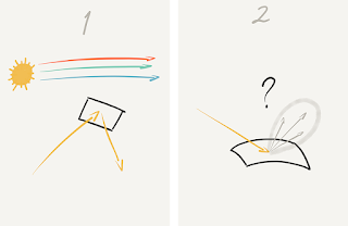
Starting from the top, we have to define our physical framework. Physics are models, made to "fit" reality in order to make predictions. Different models are appropriate for different contexts and problems. For rendering, we work with a framework called "geometrical optics".
In G.O. light is composed of multiple frequencies which are assumed to be independent. Light travels in straight lines (in homogeneous media). It changes direction at changes of media (changes of IOR), where it can be absorbed, reflected or refracted. It travels instantaneously and it follows the path of least time (Fermat's principle).
Is this a good framework? It's already making a lot of assumptions, and we know it cannot model all light behavior even when it comes to things that are easily visible: diffraction, interference, fluorescence, phosphorescence. But we say that these phenomena are not that common in everyday materials, and we might be right.
That's not all though, even before we start rendering our first triangle, we make more assumptions. First, we define a color space, usually a trichromatic one, because of the visual system metamerism. Fine, but we know that's not correct for rendering. We know spectral rendering has in even sometimes dramatically different results, but we trust our artists can tune lighting, materials, and post-processing in the right way (even if the two things shouldn't be related) to generate nice images even if we restrict ourselves to RGB. Or at least, we hope.
- Scattering
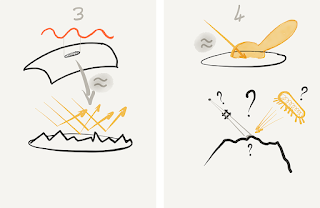
Next, we have to define what happens when the light "hits" something (an IOR discontinuity). Well, who knows, light is really hard! Some electrons... resonate? Get polarized? Please let it not be something to do with quantum stuff... Anyhow, eventually they scatter some energy back... waves? particles? There is some interference at around the atomic level. Who knows, luckily, we have another framework that comes to rescue: microfacet theory.
Surfaces are made of microfacets, like a microscopic landscape, light rays hit, bounce around and eventually come out. If we integrate the behavior of said microfacets over a small area, we can compute a scattering probability (BRDF) from the distribution of the microfacets themselves and a lot of math and voila', rendering happens.
Over a small area? How small, by the way? Well, Naty Hoffman and Eric Heitz say around the order of magnitude of the projected area of a pixel. I say, around the order of magnitude of a light wavelength, and then the projected area thing is antialiasing applied "after". So probably it's the pixel thing that's right.
What are these microfacets made of? Ideal reflectors obeying only the Fresnel law for how much light is reflected and how much refracted. The refracted part gets into the material (for dielectrics, that somehow allow this behavior), scatters some more and eventually comes out. If it comes out still "near enough" we call that "diffuse" reflection.
Otherwise, we call that subsurface scattering. But how does the light scatter inside the material? It hits particles. Microflakes? But microfacet based diffuse models (e.g. Oren-Nayar) simply swap the facets from ideal reflectors to ideal diffusers (Lambert)...
Regardless. We know all these things! We have blog posts, Siggraph talks, and books. Physics... And this still is well in that "geometrical optics" framework. Rays of light hit things. So much so that we can create raytracers to brute-force these microscopic interactions and create our own BRDFs!
But, it is still reasonable to use geometrical optics for these interactions? They seem to be quite... small. Maybe diffraction now matters? It turns out, it does, and it's a well-known thing (if you read the papers from the sixties... Beckmann-Spizzichino), but we sweep it under the rug.
And well, we can't really derive the equations from the microfacets, that integral is itself hard, so the BRDFs that we use introduce, typically, a bunch of other assumptions. For example, they might disregard the fact that light can bounce around multiple times before "coming out".
But who cares, nice pictures can be generated with this theory, and that's what matters. Moreover, someone did try to fit the resulting equations to real-world materials, right? The MERL database? I wonder how much error there is in that. Or how much it samples "well" real-world materials. Or how perceptual is the error metric used in estimating the error... Better to not think too much.
- Fiat Lux!
Are we done now? Far from it! In practice, we cannot just use the BRDF and brute-force light rays, not for real-time rendering, we're not Arnold. We need to compute a few more integrals!
We need to integrate over the light source, and over the surface area that is "seen" by the pixel, we're considering (pixel footprint). And that is incredibly hard, so hard we don't even try before having introduced a bunch more assumptions and approximations.
First of all, when we talk about pixel footprint, we really mean that we consider some statistics of the surface normals. We don't consider the fact that, for example, the "view rays" themselves change (and the light ones too), or that the surface normals don't really exist as an entity separate from actual surface geometry (which would cause shadowing and all other fun things). We assume these effects to be small.
Then, when we talk about light, we mostly mean simple geometric shapes that emit light from their surface. For example, a sphere. At each point, the light is emitted equally in all directions, and most often, it's also emitted with the same intensity over the surface.
And even then it's not enough to compute everything in closed-form. In fact, the more complex the light is, typically, the more approximated the BRDF will become. And then we'll fit these approximated BRDFs to the "real" one, and sum everything up. And sprinkle some of that pixel footprint thing on top somehow as well, but really that's done once on the "real" BRDF, even if we never actually use that!
So we have an approximation for very small lights, and maybe a good one for spheres, one for lines and capsules with some more handwaving, even more for polygonal lights, especially if textured and lastly one for far, "environment" light... We have approximations for "diffuse" and for "specular", for each of these. And maybe for static versus dynamic objects? A lot of math and different approximations.
We compare them and make sure that more-or-less the material looks the same under different kinds of light, and call it a day... The most ambitious of us might even export a scene to a path-tracer and compute some sort of ground-truth, to visually make sure things are at least reasonable...
We compare them and make sure that more-or-less the material looks the same under different kinds of light, and call it a day... The most ambitious of us might even export a scene to a path-tracer and compute some sort of ground-truth, to visually make sure things are at least reasonable...
- We're done, right?
So... we get our final image. In all its Physically Based, 60fps, HDR glory! Spectacular.
Year after year people come up with better equations, tighter approximations, and we make shinier pixels as a result.
Year after year people come up with better equations, tighter approximations, and we make shinier pixels as a result.
Is that all? Of course not! We are just getting started!
In practice, materials are not just one surface... They can have layers! And they are never optically uniform! They sparkle! They are anisotropic, they have scratches. Really, look around, look at most things. Most things are sparkly and anisotropic, due to the way they are fabricated.
And nothing is a surface, really. It's mostly volume and particles. Even... air! So we need fog and volumetric models. But that's not just about the light that scatters in the air back to our virtual cameras, we should also consider how this scattering affects lighting at surfaces. Our rays of light are not that straight anymore! Participating volumes make our light sources more "diffuse". Bigger. All of them, also things like environment lighting! And... that should affect shadows too right?
And now that we think about shadows... all this complexity and unknowns are still only for what we call "direct" lighting! What about global illumination? What about the million other hacks and assumptions that we rely upon to render each or our frames?
- Conclusions
So. How much physics is there in a frame, really? And more importantly, what's the point of all this? Should we be ashamed of not knowing physics that well? Should we do physics more? Less?
I don't know. I personally do not know physics well and I'm not too ashamed. A lot of what we've been doing is reasonable, really. We went with GGX because its "tail" helps. All the lighting improvements served our products. All the assumptions, individually, looked reasonable.
But, there is a value I think in looking at our math and our approximations holistically, now that we are getting so good at photorealism.
Perhaps there is not too much value for example in going off the deep end of complexity when we think of BRDFs, if we can't then integrate them with complex lighting, or, in order to do so, we have to approximate them again.
Similarly, the features we focus on should be evaluated. Is it more important to have non-uniform emission in our light sources, or a different "tail" in GGX/T-R? Anisotropic surfaces or sparkles? Spectral sampling? Thin-film? Non-lambertian diffuse? Of which kind? Accurate energy conservation or multi-bounce in microfacets?
Is it better to use the best possible approximation for a given integral, even if we end up with many different ones, or should we just use a bunch of spherical gaussians, or LTCs and such, but keep the same representation everywhere? And in general, is most of our error still in the materials, or in the lights? This is very hard to tell from just looking at artist-made pictures, because artists will compensate any way they can!
But even more importantly - How much can we keep relying on simplifying assumptions in order to make our math work?
I suspect to answer these questions we'll need more data. Acquire from the real world. Brute force solutions. Then look at the data and understand what matters, what matters perceptually, what errors are we committing end-to-end, and what we should approximate better and how...
And we should not assume that because somewhere we have a bit of physics, we are doing things correctly. We are, after all, a field that forgot for decades basic things like color spaces and gamma.
And we should not assume that because somewhere we have a bit of physics, we are doing things correctly. We are, after all, a field that forgot for decades basic things like color spaces and gamma.


